Zdt optimisation problem¶

In applied mathematics, test functions, known as artificial landscapes, are useful to evaluate characteristics of continuous optimization algorithms, such as:

Convergence rate.
Precision.
Robustness.
General performance.

Note

The full code for what will be proposed in this example is available: ZdtExample.py.

Rosenbrock’s function¶

In mathematical optimization, the Rosenbrock function is a non-convex function, introduced by Howard H. Rosenbrock in 1960, which is used as a performance test problem for optimization algorithms.

Mathematical definition¶

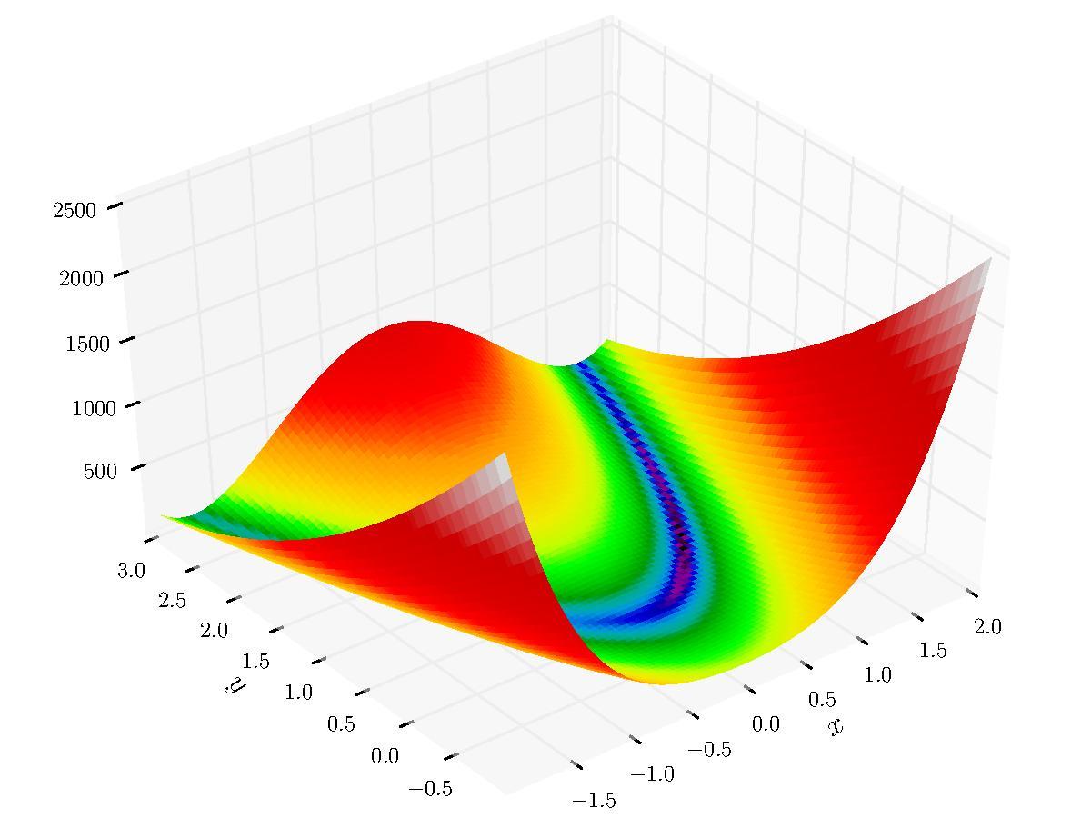
The function is defined by: \(f(x, y) = (a − x)^2 + b(y − x^2)^2\)

It has a global minimum at \((x, y) = (a, a^2)\), where \(f(x, y) = 0\). Usually these parameters are set such that \(a = 1\) and \(b = 100\). Only in the trivial case where \(a = 0\) the function is symmetric and the minimum is at the origin.

Below is a 3D representation of the function with the same parameters \(a = 1\) and \(b = 100\).

3D representation of Rosenbrock's function

The search space is defined by: \(-\infty \leq x_i \leq \infty, 1 \leq i \leq n\)

Optimal solution is defined by: \(f(1, ..., 1)=0\) when \(n > 3\)

Specific instance used¶

Using \(a = 1\) and \(b = 100\), the function can be re-written:

\(f(x)=\sum_{i=1}^{n-1}{[(x_{i + 1} − x_i^2)^2 + (1 − x_i)^2]}\)

For the current implementation example, the search space will be reduced to \(-10 \leq x_i \leq 10\) and the instance size will be set to \(n = 10\).

Macop implementation¶

Let’s see how it is possible with the use of the Macop package to implement and deal with this Rosenbrock’s function instance problem.

Solution structure definition¶

Firstly, we are going to use a type of solution that will allow us to define the structure of our solutions.

The available macop.solutions.continuous.ContinuousSolution type of solution within the Macop package represents exactly what one would wish for. I.e. a solution that stores a float array with respect to the size of the problem.

Let’s see an example of its use:

from macop.solutions.continuous import ContinuousSolution

problem_interval = -10, 10
solution = ContinuousSolution.random(10, interval=problem_interval)
print(solution)

The problem_interval variable is required in order to generate our continuous solution with respect to the search space. The resulting solution obtained should be something like:

Continuous solution [-3.31048093 -8.69195762 ... -2.84790964 -1.08397853]

Zdt Evaluator¶

Now that we have the structure of our solutions, and the means to generate them, we will seek to evaluate them.

To do this, we need to create a new evaluator specific to our problem and the relative evaluation function:

\(f(x)=\sum_{i=1}^{n-1}{[(x_{i + 1} − x_i^2)^2 + (1 − x_i)^2]}\)

So we are going to create a class that will inherit from the abstract class macop.evaluators.base.Evaluator:

from macop.evaluators.base import Evaluator

class ZdtEvaluator(Evaluator):
"""Generic Zdt evaluator class which enables to compute custom Zdt function for continuous problem

- stores into its `_data` dictionary attritute required measures when computing a continuous solution
- `_data['f']` stores lambda Zdt function
- `compute` method enables to compute and associate a score to a given continuous solution
"""

def compute(self, solution):
    """Apply the computation of fitness from solution
    Args:
        solution: {:class:`~macop.solutions.base.Solution`} -- Solution instance

    Returns:
        {float}: fitness score of solution
    """
    return self._data['f'](solution)

The cost function for the zdt continuous problem is now well defined but we still need to define the lambda function.

from macop.evaluators.continuous.mono import ZdtEvaluator

# Rosenbrock function definition
Rosenbrock_function = lambda s: sum([ 100 * math.pow(s.data[i + 1] - (math.pow(s.data[i], 2)), 2) + math.pow((1 - s.data[i]), 2) for i in range(len(s.data) - 1) ])

evaluator = ZdtEvaluator(data={'f': Rosenbrock_function})

Tip

The class proposed here, is available in the Macop package macop.evaluators.continuous.mono.ZdtEvaluator.

Running algorithm¶

Now that the necessary tools are available, we will be able to deal with our problem and look for solutions in the search space of our Zdt Rosenbrock instance.

Here we will use local search algorithms already implemented in Macop.

If you are uncomfortable with some of the elements in the code that will follow, you can refer to the more complete Macop documentation that focuses more on the concepts and tools of the package.

# main imports
import numpy as np

# module imports
from macop.solutions.continuous import ContinuousSolution
from macop.evaluators.continuous.mono import ZdtEvaluator

from macop.operators.continuous.mutators import PolynomialMutation

from macop.policies.classicals import RandomPolicy

from macop.algorithms.mono import IteratedLocalSearch as ILS
from macop.algorithms.mono import HillClimberFirstImprovment

# usefull instance data
n = 10
problem_interval = -10, 10
qap_instance_file = 'zdt_instance.txt'

# default validator (check the consistency of our data, i.e. x_i element in search space)
def validator(solution):
    mini, maxi = problem_interval

    for x in solution.data:
        if x < mini or x > maxi:
            return False

    return True

# define init random solution with search space bounds
def init():
    return ContinuousSolution.random(n, interval=problem_interval, validator)

# only one operator here
operators = [PolynomialMutation()]

# random policy even if list of solution has only one element
policy = RandomPolicy(operators)

# Rosenbrock function definition
Rosenbrock_function = lambda s: sum([ 100 * math.pow(s.data[i + 1] - (math.pow(s.data[i], 2)), 2) + math.pow((1 - s.data[i]), 2) for i in range(len(s.data) - 1) ])

evaluator = ZdtEvaluator(data={'f': Rosenbrock_function})

# passing global evaluation param from ILS
hcfi = HillClimberFirstImprovment(init, evaluator, operators, policy, validator, maximise=False, verbose=True)
algo = ILS(init, evaluator, operators, policy, validator, localSearch=hcfi, maximise=False, verbose=True)

# run the algorithm
bestSol = algo.run(10000, ls_evaluations=100)

print('Solution for zdt Rosenbrock instance score is {}'.format(evaluator.compute(bestSol)))

Continuous Rosenbrock’s function problem is now possible with Macop. As a reminder, the complete code is available in the ZdtExample.py file.